Originally we had designed the game around a compressed-distance concept where 1nm = 1km. While the intent was for faster gameplay, we quickly found some issues particularily pertaining to the speed with which engagements happen at modern speeds. This approach also necessitated some internal recalculations particularily as we use a global world with longitude/latitude coordinates for reference, and generally became rather confusing, so the decision was made to scrap distance compression altogether and simply make the world 1:1 scale. We originally had a rather short draw distance, and this had the unintended side-effect of making our environments look a lot more bland due to the fact that terrain features are now spread out over twice the distance. The solution was to increase draw distance two-fold, and it became necessary to rethink the way we approach our terrain.
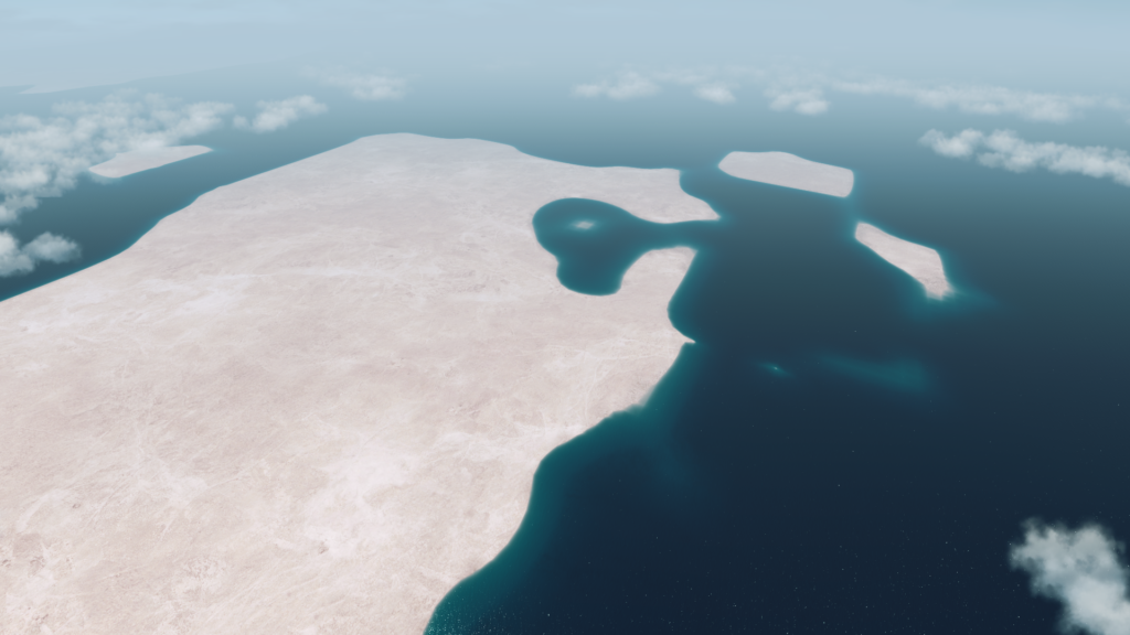
As previously mentioned in the very first dev diary, we use publicly available Digital Elevation Data that comes in 30 arc second resolution, which works out to about 1km per pixel. There is a 90m per pixel SRTM (Shuttle Radar Topology Mission) available, but this dataset is known to be noisy, doesn’t cover the polar regions at all, and would severely increase the size of the game on disc. One of the issues with the raw data is that coastlines end up jagged, and very low coastal areas end up a mess of artefacts. Again, maybe acceptable through a periscope, but awful when seen from high altitude:
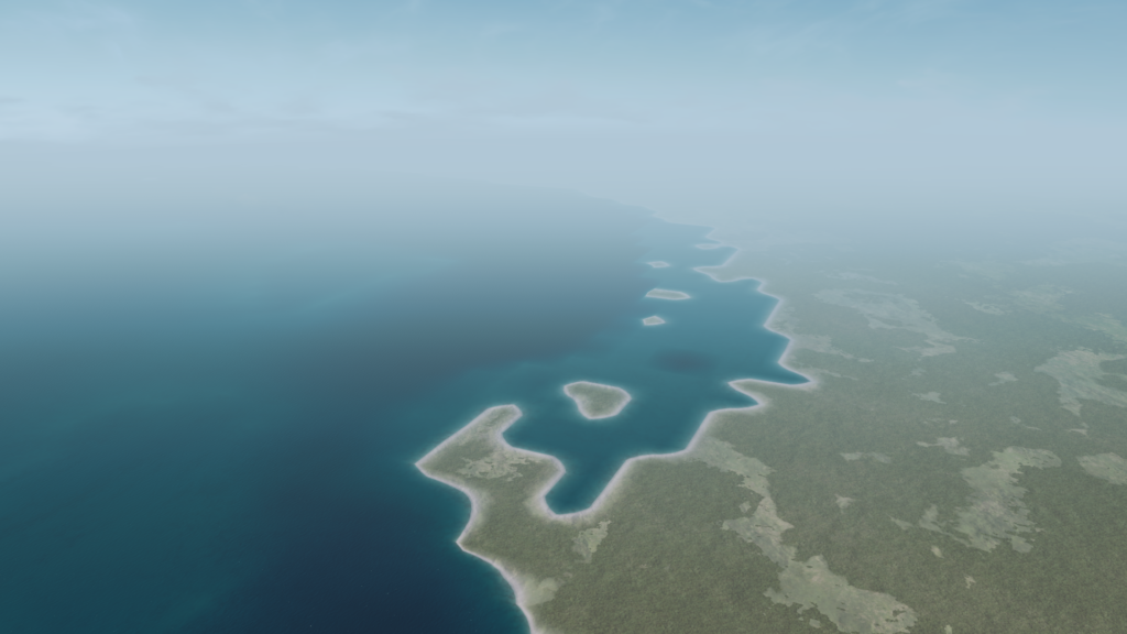
Nils and Martin tried several code-based approaches to fix the coastlines, but in the end the solution turned out to be some manual editing of the raw data in photoshop and a much better interpolation function:
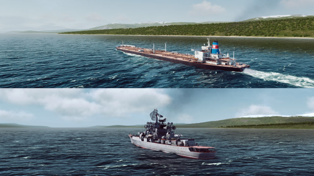
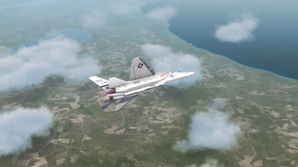
To solve the problem with featureless scenery, we elected to use publicly available landclass data employed as per-tile splat maps, with elevation being used to determine onset of permanent snow and the upper tree line – which is also modified by latitude, so you will find that in Norway, mountains show snowcaps and vegetation ends much lower than in the Vietnamese highlands, which are forest-covered. The farmland and vegetation differ between regions, and Przemek has been painting some really nice fields to fly over, and the vegetation system was adapted to differentiate between ‘wild’ vegetation and agricultural areas, so where there is farmland we can now have nice hedgerow landscapes where appropriate:
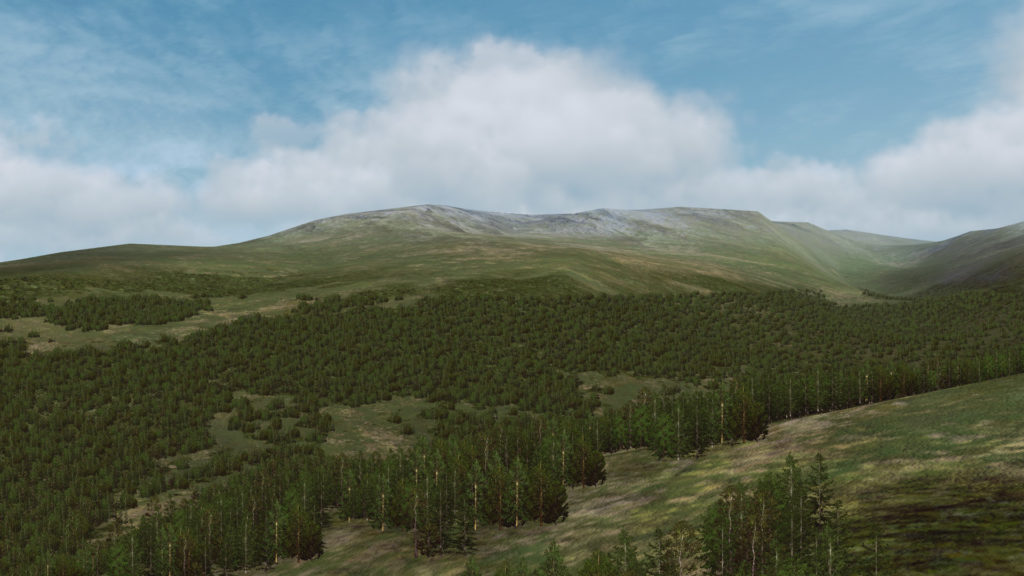

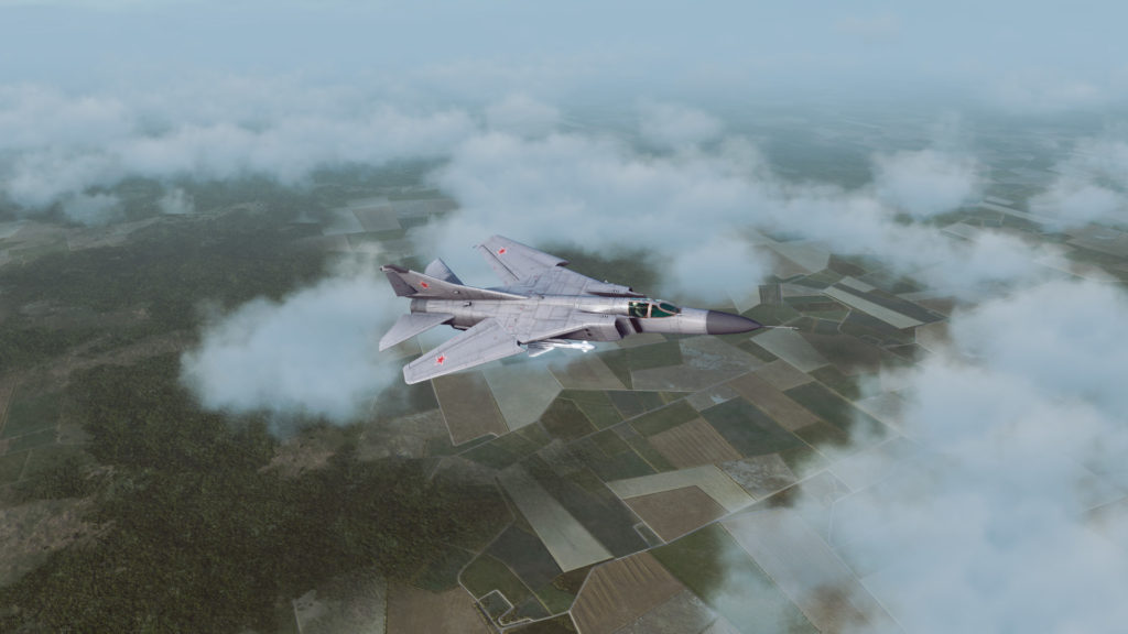
The final features to be added to the scenery are waterbodies such as lakes and rivers, and cloud shadows on the terrain. We’d like to think the final result looks better than what we had before:
We also took the step to implement ingame terrain and scenery editing tools. These allow us (and you!) to edit the terrain heightmap and place scenery objects at runtime, aiming for what you see is what you get. Note that the editor UI will be reworked in the style of the game UI prior to release:

But that’s not all, folks!
We’ve also implemented our radar model, and I will let Martin take over from here on:
Being a former radar operator who worked both with Soviet search radars (P-35) and later RRP 117 (a variant of the US AN/FPS-117 Long Range Solid-State Radar) this felt like coming home!
Proper sensor modelling is one of the most important topics for any war game as it makes the difference between survival or loss of your own units. As real sensor computation is pretty time consuming we decided to go with a model using so called RCS values (Radar Cross-Section). Those RCS values basically measure how detectable an object is by radar. It depends mainly on factors like material, the size of the target and the angle to the radar transmitter plus some other things I don’t want to go into detail here. Every object in game will have such a RCS value.
Radar image creation
So how is that radar image created using RCS?
For every search radar on any vessel/aircraft we collect all RCS values of objects which are in range. In range means here the radar horizon based on the height of the radar plus the height of the target plus minimum and maximum reachable height values for the radar itself.
These raw RCS values are now altered depending on the distance to the target where the reflected energy is multiplied with 1/distance². Additionally the heading of the target in relation to the radar transmitter is taken into account – the so called target aspect. Meaning that a broadside ship will reflect more than a bow/stern angled one. The used frequency band is another factor taken into account, especially when it comes to things like OTH (over the horizon) radars which use low frequencies which obviously comes at the cost of accuracy.
Now all these radar echoes are filtered in a way that the radar resolution is taken into account. There are two main factors:
a) the beam width which is responsible for the angular/lateral resolution
b) the pulse length which is responsible for the range/axial resolution
The axial resolution will be always the same, no matter how close the target is while the lateral resolution depends on the distance as well due to the beam width. At larger distances the lateral resolution becomes worse.
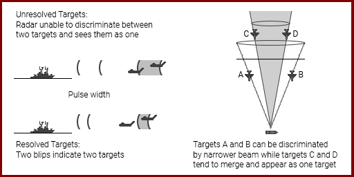
Using that information the previously collected radar echoes are now clustered/merged into “real” radar echoes that each particular radar system would see. That means that it’s very possible that your radar just shows one new contact where there are actually a cluster of 2 or 3 real contacts. Launching a Harpoon at that contact could lead to the situation where the active radar seeker of the Harpoon suddenly sees more than just one contact when closing the range. In that case it will use the brightest echo as the target which might not be the one you actually wanted to hit!
Data link
In your task force you will have data links so all sensor imagery of all your taskforce units will be combined into one sensor image. This has the big advantage for you as some of your units could be within the radar resolution to distinguish between close together contacts, so the limitations of just one radar will be resolved that way. This is done automatically for you so you will always see the best possible sensor image of your entire task force – of course based on your EMCON settings. Yet it could very well be that you cannot resolve all real targets or even see all of them.
Here’s an example of how you will see contacts on the minimap. You can see two contacts initially and then a third one appears which actually was there all the time but too close to the right one.

As you can see as soon as the new contact moves close to the left one it is now recognized as just one. But as there already was a known contact it’s now visualized in grey and the last movement is extrapolated for another 30 seconds. If it doesn’t re-appear after that time, that contact is considered to be lost.
Outlook
That’s it from the active radar side. Active sonar will be handled kind of similar, even though there are some different parameters like speed of sound and thermal layers. Passive radar and sonar will play an important role as well as ECM to jam your enemy.
Thanks for reading, more to come soon!